Beyond Attention as a Graph

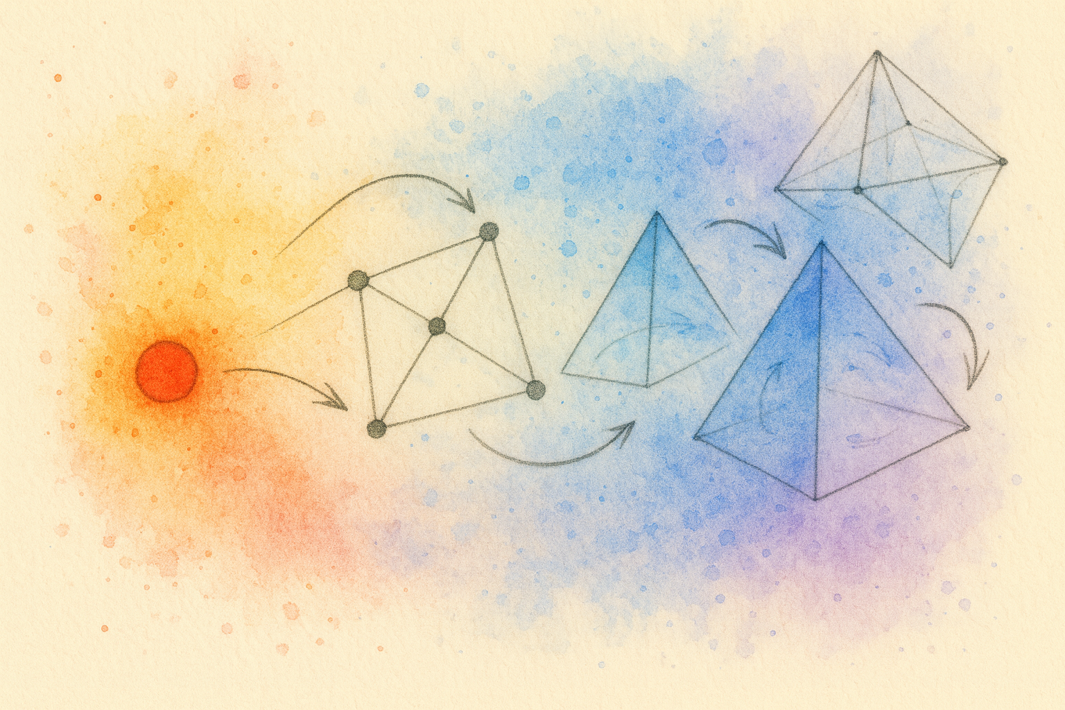
Higher-order (n-simplicial) attention as topology-driven message passing beyond graphs.

Most attention variants have been designed to retain as much sample efficiency as possible, under the constraint of achieving subquadratic scaling with respect to sequence length.

While this has clearly been a powerful research direction, recent changes in the pretraining paradigm have directed attention to architectures capable of increasing sample-efficiency.

In my previous blogpost I had briefly introduced, as a tool to explain attention sinks, a simple way of viewing attention as a graph operation.

We will use this same viewpoint to argue that regular transformers may be fundamentally limited in their message-passing capabilities, arguing in favor of higher-order attention methods, such as 2-simplicial Attention and provide a natural way of generalizing it to $n$-simplices, while explaining them from a topological perspective.

Finally, we will also poke at the very mechanism that makes Machine Learning “deep”: layer composition.

Motivation

“Deep Learning” is named after the typical definition of Neural Network models as a set of subsequent, composed Layers.

Layers represent atomic, parametric transformations between vector spaces, rendered non-linear by a selection of activation functions.

In transformers, layers are organized in transformer blocks, and the two are often used interchangeably. Transformer blocks are nothing more than subsequent attention and MLP transformations operating on the residual stream.

Intuitively, depth is easy to justify: while the Universal Approximation Theorem guarantees that a single, infinitely wide non-linear layer can approximate any continuous function arbitrarily well, it doesn’t mean that width scaling is practical.

As it turns out, properly approximating functions becomes exponentially hard with respect to the dimension of the spaces the functions map between, which can be seen as another angle of the curse of dimensionality.

For this reason, it becomes convenient to instead “break down” the approximation problem by composing several parametric layers, one after the other.

This allows the model to increase in expressivity without exploding in (latent) dimensionality.

As for all worthwhile architectural choices in deep learning, this exposes us to a tradeoff: composing operations sequentially is by definition the least parallel (and hence fast) architectural choice we can make.

Depth for Transformers

While the previous considerations apply in general for all Neural Network architectures, transformers in particular have their specific drawbacks when scaling depth: Transformers’ success has been greatly propelled by their natural parallelism during Next Token Prediction tasks, and, apart from inevitably increasing latency in both inference and training, depth exposes the network to further instability in gradients, as, depending on normalization, the model risks vanishing or exploding gradients.

In sequence modelling, though, one key element justifies depth: attention is an operation that message-passes between pairs of tokens in a graph. This means that individual transformer blocks can only possibly encode interactions between pairs of tokens. Depth allows information to be passed beyond a single-hop: if we reframe the $AV$ multiplication as in the attention sinks blogpost (seeing as “diffusion” of $V$ on the graph), we can reconnect this intuition to regular graph theory by noticing how powers of the adjacency matrix of a graph, $A^k$, represent $k$-hop walks from each node, and therefore depth approximates this due to attention’s fully connected, yet sparse, input-dependent adjacency matrix.

As a result, depth is a fundamental ingredient in transformers that allows them to effectively message-pass between tuples of tokens, and hence build complex and useful representations of tokens in sequences.

But what if there existed a way to message-pass between tuples of tokens without resorting to depth?

What lies beyond graphs

As we know, the message-passing operation happening during attention can be conceptualized as a graph operation. This simple observation, while trivial, has a relevant practical consequence: an entire field of science has, since roughly 2017, been extensively studying Neural Networks as message-passing on graphs, and has developed a variety of theories and techniques to best represent information on topological objects. Of course, the field in question is Geometric Deep Learning, and its central contributions, Graph Neural Networks and Topological Deep Learning.

Notably, one key element of that vast literature has been an expressivity bound on GNN architectures: if we define “expressivity” as the capability of distinguishing graphs that are different, then a GNN is only as expressive as the Weisfeiler-Lehman test (also referred to as the WL-test) . I won’t go in the details of what the test is, and will gladly refer the interested reader to Federico Barbero’s excellent video explaining it.

If you don’t have the time, here’s the gist of it: the WL-test is designed to understand when two graphs are isomorphic (the same graph), but it doesn’t always work. It can be shown that a GNN is at most as expressive at graph ismorphism as the WL-test itself.

If you’re anything like me, this sounds like bad news: what do you mean we have a theoretically bounded expressivity? Isn’t universal approximation the reason we like Neural Networks so much?

Fortunately, not everything is lost. As it turns out, it’s possible to “break” the WL-test bound by inserting higher-order topological information.

But what does it mean?

As you know, a graph is a pair $\mathcal{G} = (\mathcal{V}, \mathcal{E})$ , where $\mathcal{V} = {1, 2, \cdots , n}$ is a set of nodes, and $\mathcal{E}: \mathcal{V} \times \mathcal{V} \rightarrow {0,1}$ is a set of links, also called edges if $(i,j) \in \mathcal{E}$ also implies $(j,i) \in \mathcal{E}$.

In other words, elements in $\mathcal{E}$ represent directed, pairwise relations between nodes in the graph.

This can be naturally extended by considering a generalization of $\mathcal{E}$, say $\mathcal{E}^{(k)}$, with $k \in \mathbb{N}$, where \(\mathcal{E}^{(k)} : \mathcal{V}^{k+1} \rightarrow \{0,1\}.\)Intuitively, this represents $k$-sized tuples of nodes. For example, for $k=2$, this is equivalent to all directed triangles between nodes, while the case $k=1$ recovers the original graph with pairwise links. Note, how, intuitively, for $\mathcal{E}^{(k)}$, we would be effectively considering $k$-dimensional$\,$geometric objects: nodes would be 0-dimensional points, edges 1-dimensional lines, triangles 2-dimensional surfaces, and so on (of course this is just an intuition, for this to be true we would need to embed our nodes in a space and require relations to be undirected).

Inserting higher-order information in message passing in GNNs can be shown to increase expressivity beyond the regular WL-test. More generally, it can be shown that the networks with order $k$ topological information are bounded by the $k$-WL test.

While this is by no means a formal introduction to higher-order topological objects like Simplicial Complexes, it should be sufficient to paint an intuition about where we’re going: if we manage to message-pass also considering higher order topological objects, instead of just pairs of tokens, we may be able to capture more complex patterns in parallel, instead of having to rely on depth.

2-Simplicial Attention

The Higher-order Attention idea has been floating around for a while: its first implementation in a transformer architecture is dated to the 2019 work by Clift et al., and further along has been reinvented/reinterpreted/tangentially rediscovered in a series of works, such as Representational Strengths and Limitations of Transformers, Tensor attention , The Cellular Transformer, AlphaFold 2, TransNAR and i’m sure a bunch of others. Even I, since last year, have been obsessed with the idea, proposing it in public a couple of times.

Apart from theoretical work, what this idea really needed was a step towards experimental validation under a modern paradigm. Fortunately, Aurko, Rohan and their colleagues delivered well beyond that: a novel implementation of an Higher-order Attention method was the first architectural change to seem to induce a change in the exponent in the scaling law of Large Language Model.

Fig. 1: scaling law results from the Fast and Simplex: 2-Simplicial Attention in Triton paper.

Rediscovering Simplicial Attention from the Topological Perspective

So, how do we extend our graph-based perspective on attention, so that it naturally becomes a (potentially higher-order) topological perspective?

Refreshing the graph case, let’s take, for example \(X \in \mathbb{R}^{\,n\times d}\)

And let’s treat the rows of $X$ as a point‑cloud: \(X = \begin{bmatrix} x_1^{\!\top}\\ x_2^{\!\top}\\ \vdots\\ x_n^{\!\top} \end{bmatrix}, \qquad x_i \in \mathbb{R}^d.\)

Constructing the $Q$,$K$,$V$ matrices for attention, we effectively project that cloud in three ways

\[Q = X W_q \in \mathbb{R}^{\,n\times d_q}\] \[K = X W_k \in \mathbb{R}^{\,n\times d_q}\] \[V = X W_v \in \mathbb{R}^{\,n\times d_v}.\]

We use these distinct projections to capture a graph-like structure, building an adjacency matrix between tokens, which can be seen as nodes \(\alpha_{ij} \;=\; \langle q_i, k_j\rangle \;=\; q_i k_j^{\!\top}, \qquad q_i = [Q]_{i,:},\; k_j = [K]_{j,:}.\) Stacking all scores: \(\alpha \;=\; Q K^{\!\top} \in \mathbb{R}^{\,n\times n}.\)

The intuition is: the more points align in Query - Key space, the stronger their connection will be, and hence the stronger the link between the nodes.

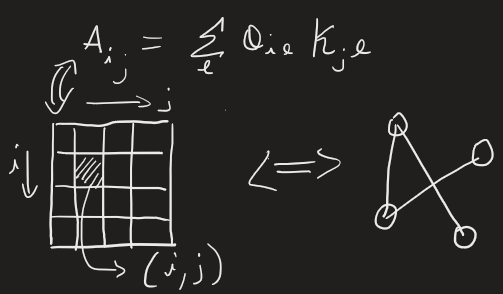
Fig 2: an attention matrix encodes a graph

Finally, we use softmax to normalize outgoing weights from each node

\[A_{ij} = \frac{\exp\!\bigl(\alpha_{ij}/\sqrt{d_k}\bigr)} {\displaystyle\sum_{j'=1}^n \exp\!\bigl(\alpha_{ij'}/\sqrt{d_k}\bigr)}\,, \qquad A = \mathrm{softmax}\!\Bigl(\tfrac{\alpha}{\sqrt{d_k}}\Bigr)\]

Each row of $A$ is a probability distribution and corresponds to the node’s neighbors; small logits shrink toward 0, meaning most edge weights are very close to zero, apart from a few. This effectively heavily sparsifies the neighborhood, assigning most of the link weights to just a few connections, while the rest go to zero.

Lastly, the final operation

\[\mathrm{attention}(x) = AV\]

can now be interpreted from an interesting perspective: $V$ can be seen as a vector-valued function defined on nodes of the graphs which is diffused from its neighbors to each node.

Fig. 3: left: central node ($i$) weighs via attention neighboring nodes; right: central node aggregates via attention weights the value function defined on neighboring nodes

But we already knew all of this from the previous blogpost. The key point to notice, here, is the operation we perform to extract a graph: we project $X$ into two distinct spaces via $W_Q$ and $W_K$, precisely because we need to perform a bi-linear form (the dot product) to extract a two-way relationship.

What if we wanted to capture three-way relationships? Naturally, one could think of adding a second $K^{\prime}$ matrix, resulting from a $W_{K^{\prime}}$ projection, such that we would have a 3D tensor \(T_{ijk} = \sum_{l}Q_{il}K_{jl}K^{\prime}_{kl}\) Which can also be seen as taking a multilinear product, if viewed per query: \(T_{ijs} = \langle q_i, k_j, k^{\prime}_s \rangle\)

Notice how, before, each attention score $A_{ij}$ represented the link weight going from node $i$ to node $j$. Now, each entry $T_{ijk}$ can instead be seen as the collective weight assigned to the triangle determined by the (directed) walk from node $i$, passing through node $j$, and ending up in node $k$.
Such a triangle, in algebraic topology, may also be called a 2-simplex (a node is a 0-simplex, an edge is a 1-simplex), explaining the naming of the attention mechanism.

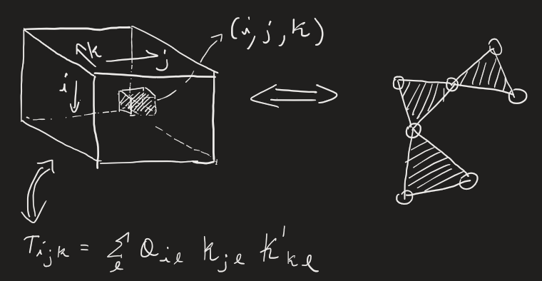
Fig. 4: 2-simplicial attention’s tensor T, in each of its entries, represents a (directed) 2-simplex (triangle)

Now that we’ve found a formulation to represents 2-simplices (or simplexes, one day i’ll have to decide which version of the plural i prefer), how do we transfer our regular sparsification mechanism (softmax) to it? And, moreover, what even is a neighborhood in this case?

The intuitive extension of attentions (also used in 2-simplicial attention) treats this by keeping the query token as central: instead of being a matrix, our attention score is now a 3D tensor. This simply means that, instead of rows, we now normalize over entire slices associated with query $i$.

Meaning, our softmax operation becomes: \(\alpha^{(2)}_{ijk}= \mathrm{softmax(T)}^{(2)}_{ijk} = \frac{e^{T_{ijk}}}{\sum_{jk}e^{T_{ijk}}}\) Intuitively, this is defining the node’s neighborhood as the triangles it’s included in. Hence, here, we’re squashing to zero triangles with low three-way similarity, and amplifying the signal from the more similar ones.

This makes sense because our final goal will be to use this information to update the nodes’ embeddings. With that said, there exist more ways to define adjacency for higher order structure: an interesting idea could be to normalize over triangles sharing faces, instead.

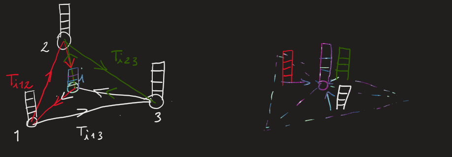
Fig. 5: left: message passing now happens between 2-simplices (oriented triangles). Each 2-simplex is weighed by an entry in tensor T. Right: each 2-simplex has an aggregated value vector that is used to update the node’s representation

The last piece of the puzzle is the $V$ matrix of regular attention. As we discussed previously, it can be thought of as a vector-valued function defined on nodes, where individual vectors are rows $V_i$.

So what about 2-simplicial attention? Naturally, $V$ would still have to be defined token-wise, but now we have to engineer it so that it can represent, for node $i$, the value associated with the neighbors in a triangle, just like in regular attention $V$ was being aggregated from neighbors in the graph. Furthermore, in order to express value of tokens with full degrees of freedom, we introduce a second value projection, $V^{\prime}$, that we use analogously to $K^{\prime}$. What we need is for all triangles $(i,j,k)$ to aggregate $V_j$ and $V_{k}^{\prime}$ with some function $f:\mathbb{R}^{h}\times \mathbb{R}^{h} \rightarrow \mathbb{R}^{h}$. such that we have, for each triangle, a resulting vector \(V^{(2)}_{ijk} = f(V_{k},V_{k}^{\prime})\). In the paper, f is just the product of the entries of $V$, which can be conveniently written as an element-wise product between $V$ and $V^{\prime}$: \(V^{(2)}_{ijk} = V_{ik}V_{jk}^{\prime}\) Apart from convenience, this choice can also be seen as combining value vectors using an “AND” operation, in the sense that large values will compound, and a single small value is sufficient to drop the magnitude of the vector. This is opposed, for example, to having the function be \(V^{(2)}_{ijk} = V_{ik}+ V_{jk}^{\prime}\) which would, instead, be analogous to an “OR” operation.

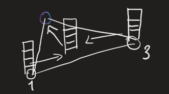
Fig. 6: $v$ and $v’$ from each triangle are aggregated and used to update the central node’s embedding

At last, we end up with $V^{(2)}$ being another 3D tensor. This allows us to perform the final operation of attention as a tensor contraction taking us back to our regular $\mathbb{R}^{n\times d}$ shape: \(\mathrm{attention(x)}_{il} = \sum_{jk}\frac{\alpha^{(2)}_{ijk}V^{(2)}_{jkl}}{\sqrt{d}}\) Note how this operation can still be thought of as some kind of “diffusion”: we are aggregating value vectors from each triangle including node $i$, scaling them and summing them to update the vector in node $i$.

Now, the extension to the n-simplicial case is trivial: For n-simplices, we just repeat the 2-simplicial recipe with $n$ Key projections. For an $(n+1)$-tuple $(i,j_1,\ldots,j_n)$ define the score tensor by a multilinear form

\[T_{i\,j_1\cdots j_n} \;=\; \sum_{\ell} Q_{i\ell}\;\prod_{m=1}^n K^{(m)}_{j_m\ell} \;=\;\langle q_i, k^{(1)}_{j_1},\ldots,k^{(n)}_{j_n}\rangle,\]

and normalize per-query over all $n$-tuples to get

\[\alpha^{(n)}_{i\,j_1\cdots j_n} \;=\; \frac{\exp T_{i\,j_1\cdots j_n}}{\sum_{(j_1,\ldots,j_n)} \exp T_{i\,j_1\cdots j_n}}.\]

Values remain token-wise but are combined along each $n$-simplex via a symmetric $n$-ary reducer $f$ ; the simplest is the element-wise product “AND”

\[V^{(n)}_{i\,j_1\cdots j_n} \;=\; \prod_{m=1}^{n} V^{[m]}_{j_m i},\]

though sum/mean (an “OR”) or MLP reducers are possible. The update is then a contraction over all $n$-tuples incident to $i$ :

\[\mathrm{attn}(X)_{i\ell}\;=\;\frac{1}{\sqrt{d}}\sum_{j_1,\ldots,j_n}\alpha^{(n)}_{i\,j_1\cdots j_n}\; \big[V^{(n)}_{j_1\cdots j_n}\big]_\ell\]

Topologically, we’re diffusing over the star of $i$ in the $n$-skeleton (cofaces incident to $i$ ), so higher-order interactions are captured in one hop.

Naturally, an $n$-simplicial attention mechanism’s memory scales catastrophically quickly with sequence length, precisely with $O(L^{n+1})$. This means that we have to come up with ways of saprsifying this mechanism in order to make it practical.

In the 2-simplicial attention paper, this is solved by performing Sliding Window Attention (SWA) with potentially different windows per dimension in the attention tensor.

But is this the only way to tackle this? When i first started pondering these ideas, my first thought was instead to route tokens dynamically to a fixed size window. A very similar idea came recently with Deepseek 3.2, in the shape of DeepSeek Sparse Attention (DSA). The intuition is simple: why have a sliding window when you can hand-pick the tokens you want to use, with your preferred sparsity?

DSA (DeepSeek Sparse Attention) replaces dense attention with a two-stage sparse mechanism: a lightweight indexer followed by top-k token selection.

The indexer computes cheap similarity scores between each query and all past tokens. For each query token $i$ and indexer head $h$, it first computes

\[s_{i j h} \;=\; \mathrm{ReLU}(\langle q^I_{i h},\, k^I_{j} \rangle) \cdot w^I_{i h},\]

where $q^I_{i h}$ is the indexer’s query vector for token $i$ and head $h$, $k^I_j$ is the (shared) indexer key for token $j$, and $w^I_{i h}$ is a learned per-head weight. Summing over heads gives the final score

\[S_{ij} \;=\; \sum_{h=1}^{H_I} s_{i j h}.\]

For each query $i$, the top-k keys according to $S_{ij}$ are selected:

\[\mathcal{K}_i \;=\; \mathrm{TopK}_j \big(S_{ij},\, k\big),\]

and full attention is then computed only on this restricted set.

This reduces the core attention complexity from $O(L^2)$ to $O(Lk)$, while preserving the most relevant interactions, making it particularly effective for long contexts.

Fig. 7: intuitively representing full attention, SWA and DSA in the regular case

In our case, we use a modified version of DSA to substitute SWA: first, we notice that substituting ReLU with softmax performs better on our small experiments on a token-wise level. Furthermore, to avoid individual computation of $qk_1^T$ and $qk_2^T$ distinct pairs, we instead leverage existing $QK^T$ from the previous regular attention layers, and directly index based on those scores, obtaining the same exact top-k scorers for both $k_1$ and $k_2$.

This yields a tiny speedup to our very small model / small token-horizon run, while keeping the same scaling as SWA, where we have $O(Lk^2)$ (with $k$ chosen to be equivalent to the window size of SWA) instead of the full sequence $O(L^3)$.

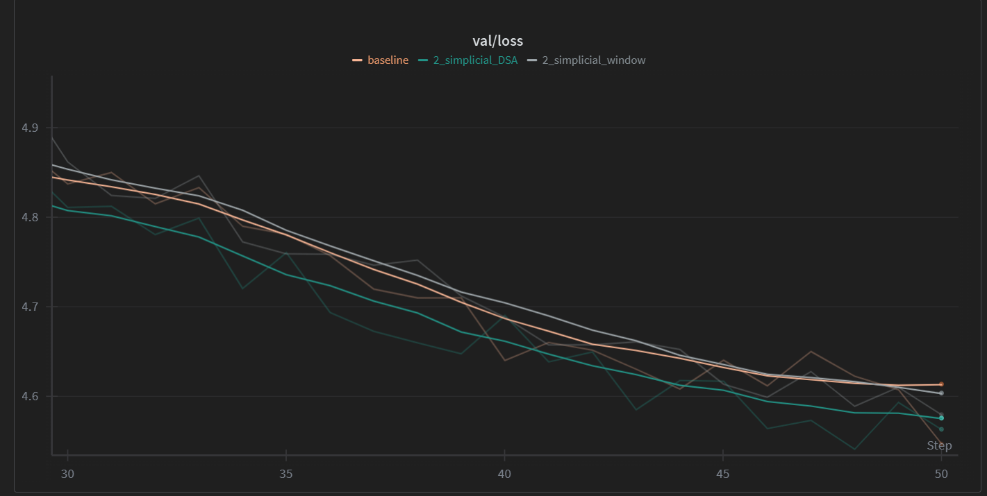
Fig. 8: losses for a 127M variant of nanogpt using a 3:1 regular to 2-simplicial attention ratio, with a block size of 512 and a top-k/SWA window of 128 tokens. In gray, is the SWA-sparsified version, in green the DSA-inspired technique we introduced. In orange, regular self-attention. Total token horizon is of around 60M tokens.

While in Fig. 8 we can see that baseline appears to have roughly the same acceleration as windowed simplicial attention, we notice how the 2-simplicial attention paper itself only notices gains against the transformer at a much larger parameter size, as seen in Fig. 10.

Overall, though, our acceleration is of an average of 0.76% (so barely noticeable) with respect to the Sliding Window Attention version. In Fig.9, we can see (batch-wise) speedup in training:

Fig. 9: speedup across steps of DSA and SWA vs baseline

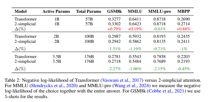
Fig.10: reported performance comparison between transformers and 2-simplicial attention in the original paper.

So what does $n$-simplicial attention mean for depth?

As we’ve discussed, one of the key elements of depth is multi-token representation-learning. Another way to view it, is that individual tokens are in a constant relay race: each token wants to get to a target representation, but needs crucial information from other tokens’ representations to do so. If the proper representation is very hard to find, the model eventually runs out of depth to message-pass. 2-simplicial attention goes in the direction of fixing this, because it combinatorially opens up surface area for the model to do message-passing, for each block. Of course, the present one is just its first, prototypal iteration, which will inevitably change in the future (us at Gladia are already hard at work).

Wrapping up

We’ve explored a recent advance in attention architecture, and explained it using our previously established topologically-oriented angle. We’ve also outlined a trivial extension to n-simplices of the mechanism, as well as demonstrated tiny gains in expressivity by utilizing a DSA-like sparsification of 2-simplicial attention keys, substituting SWA. Given my obsession with the topic, you’re very likely to read something from me on the topic soon. In the meantime, let me know what you think!

Acknowledgements

Thanks a lot to thelakosiffers, davinci MatteoManias, Francesco Bertolotti, ueaj, Bianca, Aurko,Rohan , Mike , Borak, Berto and Niccolò Gentile for their precious feedback!

---

Suggested citation

@misc{pappone2025beyondattention,
  author       = {Francesco Pappone},
  title        = {Beyond Attention as  Graph},
  year         = {2025},
  month        = {October},
  day          = {09},
  institution  = {Università La Sapienza di Roma -- PSTP Technoscience},
  howpublished = {\url{https://publish.obsidian.md/the-tensor-throne/The+Graph+Side+of+Attention/Beyond+Attention+as+a+Graph}}, 
  note         = {Blogpost}
}